Understanding Insulin on Board (IOB) Calculations
The amount of Insulin on Board (IOB) at any given moment is a key input into the determine-basal logic, which is where all the calculations for setting temporary basal rates or small microboluses (SMBs) takes place. This amount of insulin on board gets passed into oref0/lib/determine-basal/determine-basal.js as part of the iob.json file. That information is then used to project forward blood glucose (BG) trends, which the determine-basal logic then responds to in order to correct course. This piece of the OpenAPS documentation provides an explanation of the assumptions used about how insulin is absorbed and how those assumptions translate into the insulin on board calculations used to project BG trends.
First, some definitions:
- dia: Duration of Insulin Activity. This is the user specified time (in hours) that insulin lasts in their body after a bolus. This value comes from the user’s pump settings.
- end: Duration (in minutes) that insulin is active.
end=dia* 60.
- peak: Duration (in minutes) until insulin action reaches it’s peak activity level.
- activity: This is percent of insulin treatment that was active in the previous minute.”
Click here to expand information about insulin activity calculations for older insulin curves with DIA shorter than the 0.7.0 default of 5, as well as information about current variables used in IOB calculations:
Insulin Activity
The code in oref0/lib/iob/calculate.js calculates a variable called activityContrib, which has two components: treatment.insulin and a component referenced here as actvity. The unit of measurement for treatment.insulin is units of insulin; the unit of measurement for activity is percent of insulin used each minute and is used to scale the treatment.insulin value to units of insulin used each minute. (There is no variable activity created in oref0/lib/iob/calculate.js. There is, however, a variable called activity created in oref0/lib/iob/total.js, which represents a slightly different concept. See the FINAL NOTE, below, for more details.)
There are three key assumptions the OpenAPS algorithm makes about how insulin activity works in the body:
Assumption #1: Insulin activity increases linearly (in a straight line) until the
peakand then decreases linearly (but at a slightly slower rate) until theend.Assumption #2: All insulin will be used up.
Assumption #3: When insulin activity peaks (and how much insulin is used each minute) depends on a user’s setting for how long it takes for all their insulin to be used up. That setting is their duration of insulin activity (
dia) and generally ranges between 2 and 8 hours. The OpenAPS logic starts off with a default value of 3 hours fordia, which translates into 180 minutes forend, and assumes that insulin activity peaks at 75 minutes. (This is generally in line with findings that rapid acting insluins (Humalog, Novolog, and Apidra, for example) peak between 60 and 90 minutes after an insulin bolus.) This assumption, however, is generalizable to other userdiasettings. That is,peakcan be expressed as a function ofdiaby multiplying by the ratio (75 / 180):peak= f(dia) = (dia* 60 * (75 / 180))So, for example, for a
diaof 4 hours,peakwill be at 100 minutes:100 = (4 * 60 * (75 / 180))
NOTE: The insulin action assumptions described here are set to change with the release of oref0, version 0.6.0. The new assumptions will use exponential functions for the insulin action curves and will allow some user flexibility to use pre-set parameters for different classes of fast-acting insulins (Humalog, Novolog, and Apidra vs. Fiasp, for example). For a discussion of the alternate specifications of insulin action curves, see oref0 Issue #544. When oref0, version 0.6.0 is released and the current assumptions are no longer recommended, this documentation will be updated.
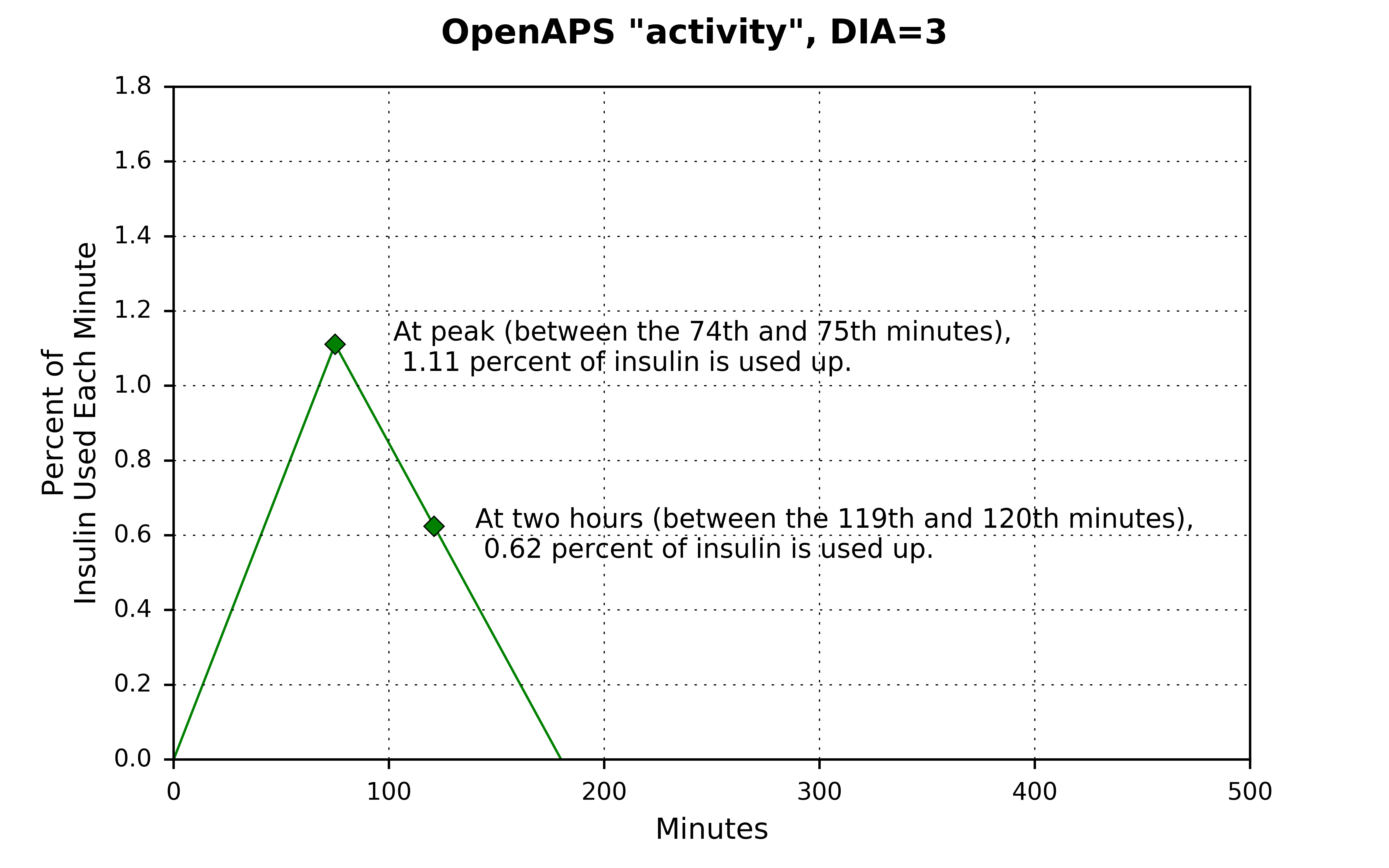
What The Insulin Activity Assumptions Look Like
Given a dia setting of 3 hours, insulin activity peaks at 75 minutes, and between the 74th and 75th minutes, approximately 1.11 percent of the insulin gets used up.
Adding up all the insulin used each minute between 0 and end, will sum to 100 percent of the insulin being used.
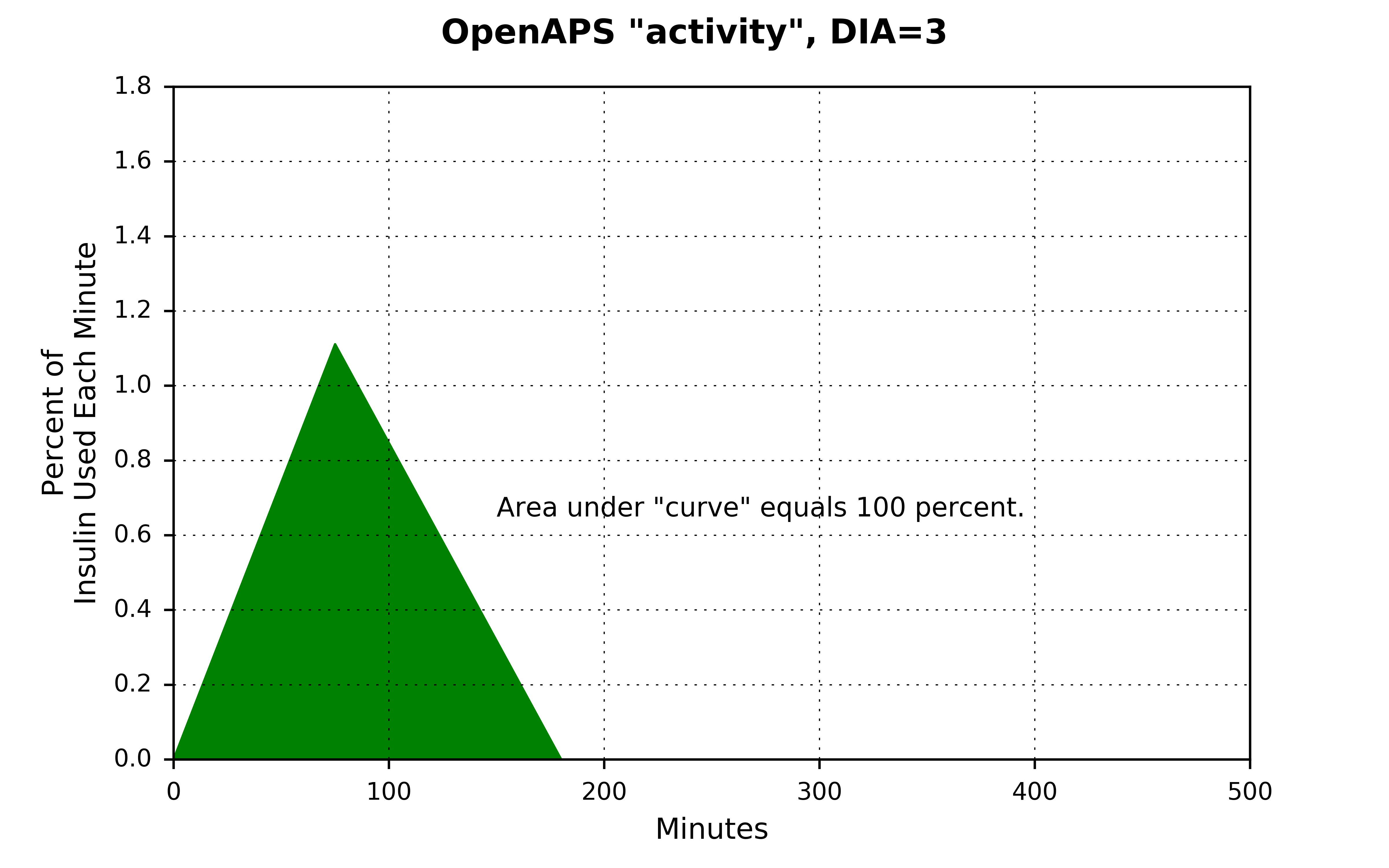
The area under the “curve” can be calculated by taking the definite integral for the activity function, but in this simple case the formula for the area of a triangle is much simpler:
Area of a triangle = 1/2 * width * height

            = 1/2 * 180 * 1.11

            = 99.9 (close enough to 100 -- the actual value for activity is 1.1111111, which gets even closer to 100)
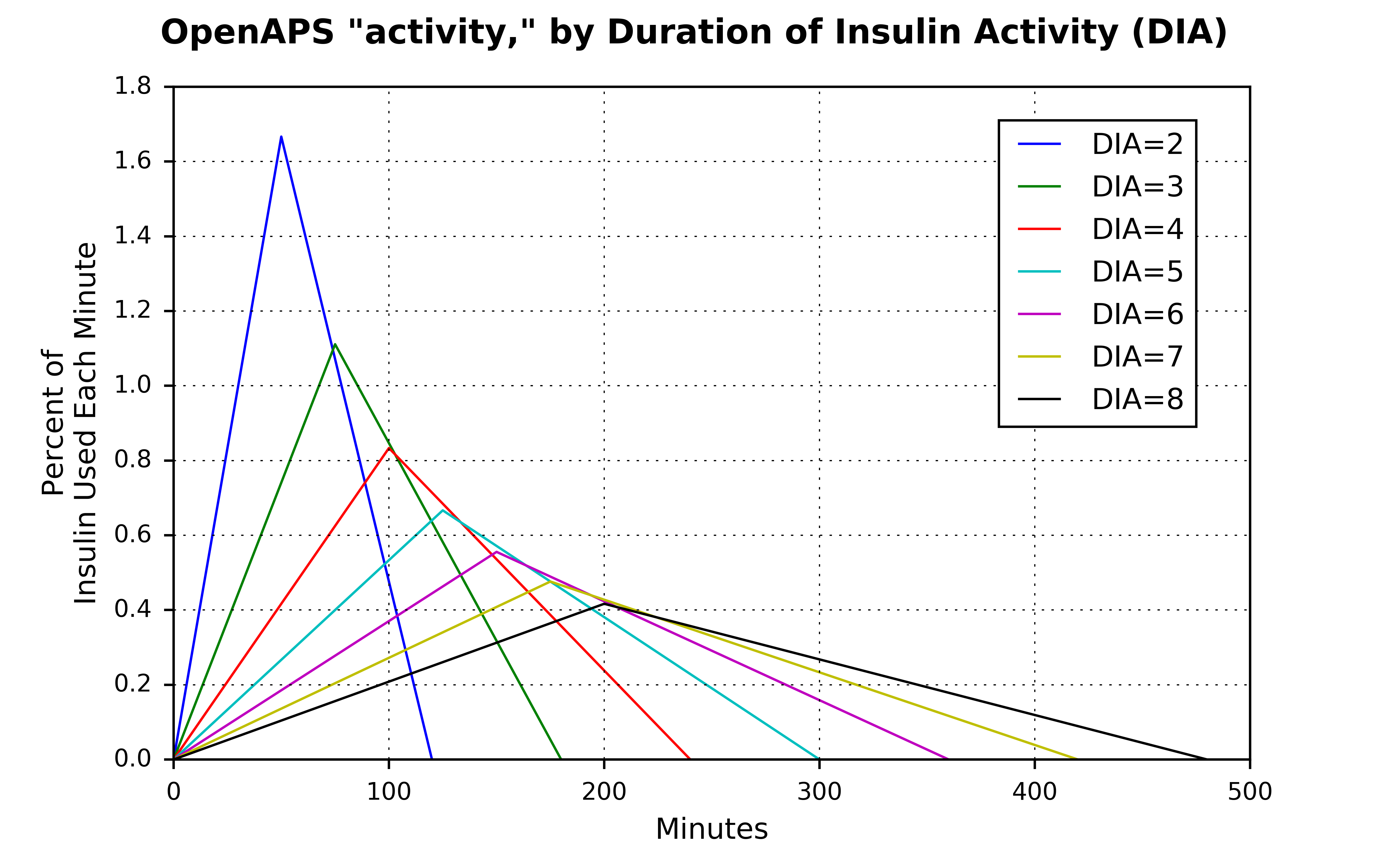
For shorter dia settings, the peak occurs sooner and at a higher rate. For longer dia settings, the peak occurs later and at a lower rate. But for each triangle, the area underneath is equal to 100 percent.
Cumulative Insulin Activity
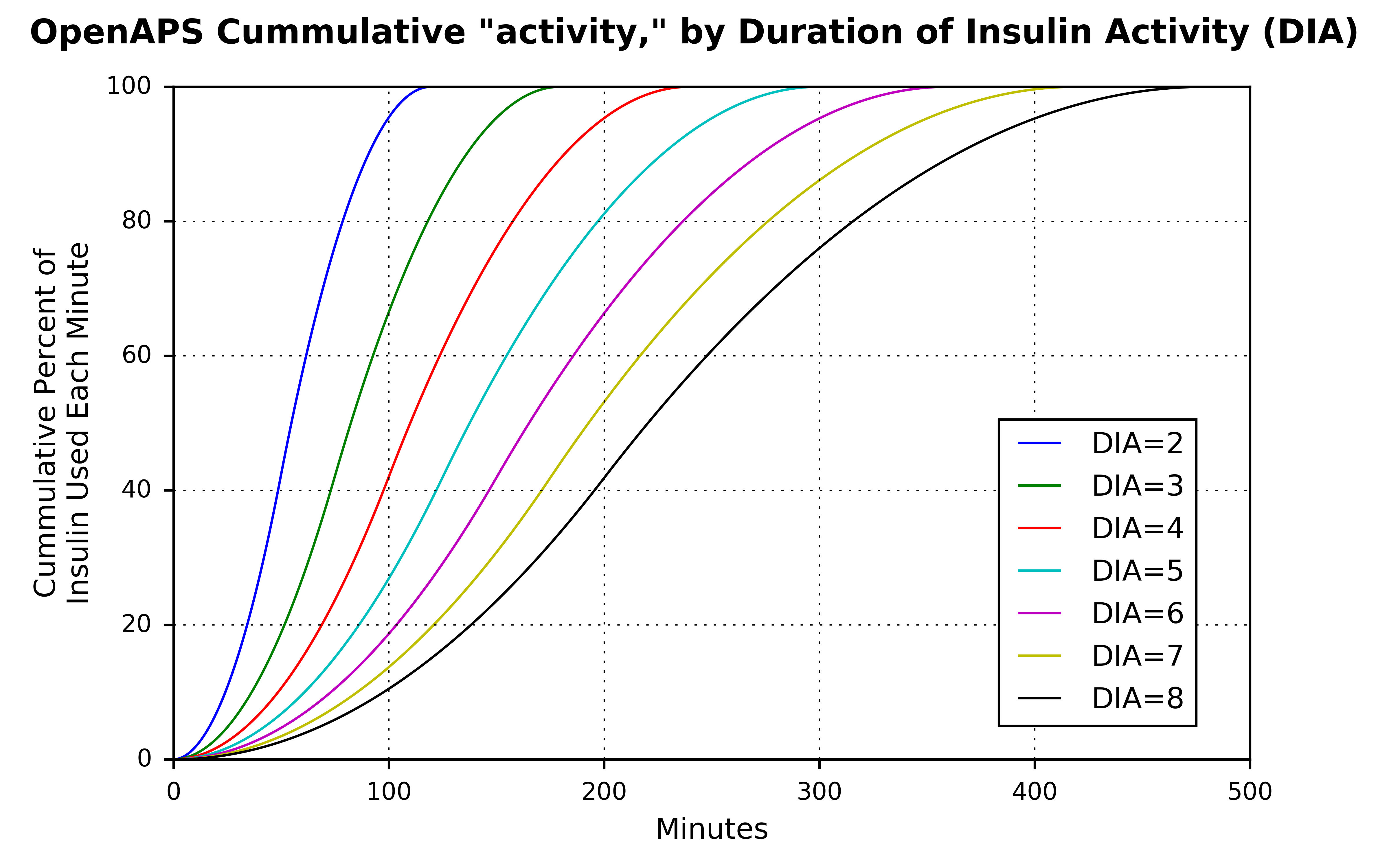
Given these activity profiles, we can plot cumulative activity curves, which are S-shaped and range from 0 to 100 percent. (Note: This step isn’t taken in the actual oref0/lib/determine-basal/determine-basal.js program, but plotting this out is a useful way to visualize/understand the insulin on board curves.)
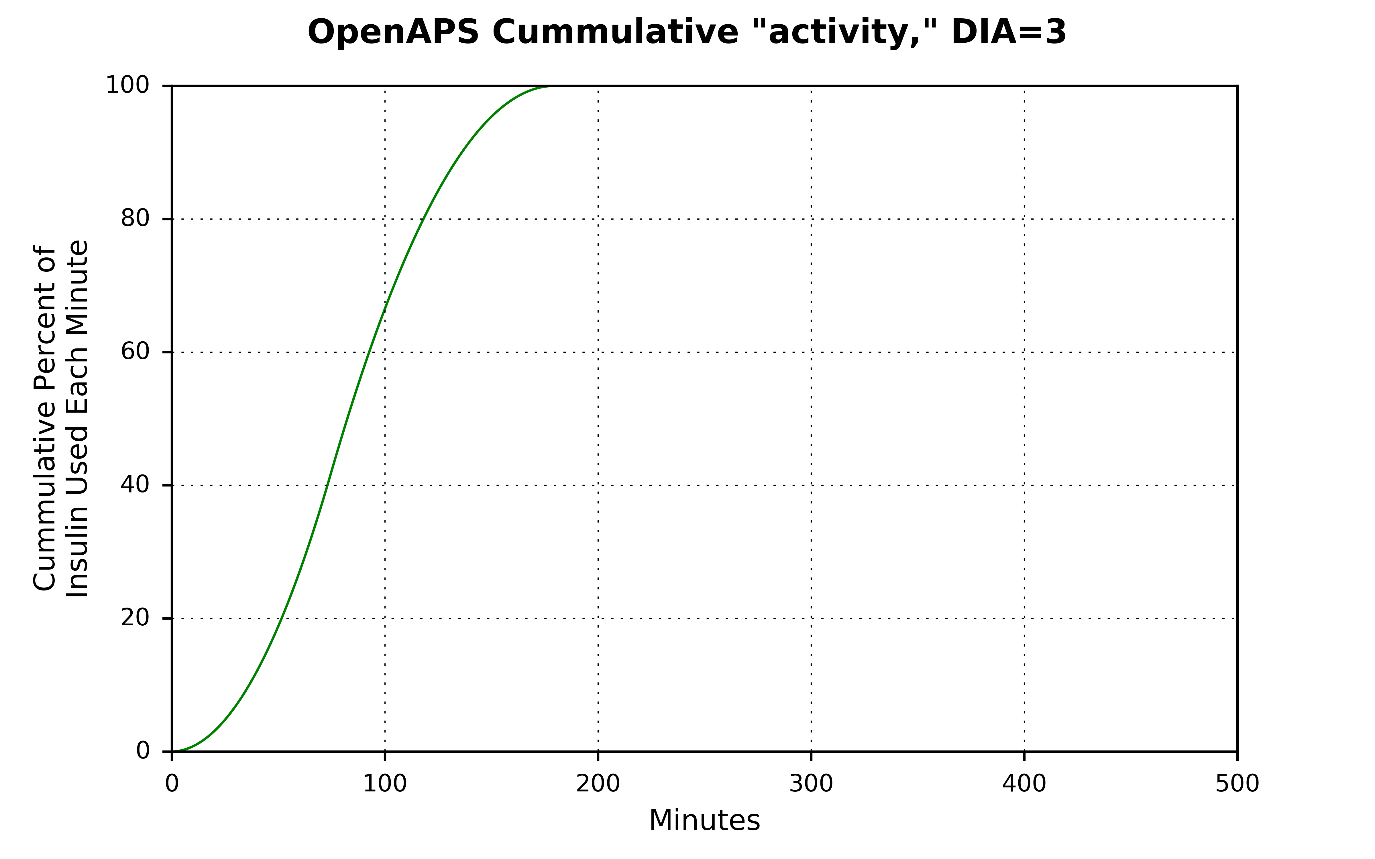
Just like how the insulin activity curves shift depending on the setting for dia, the cumulative activity curves do as well.
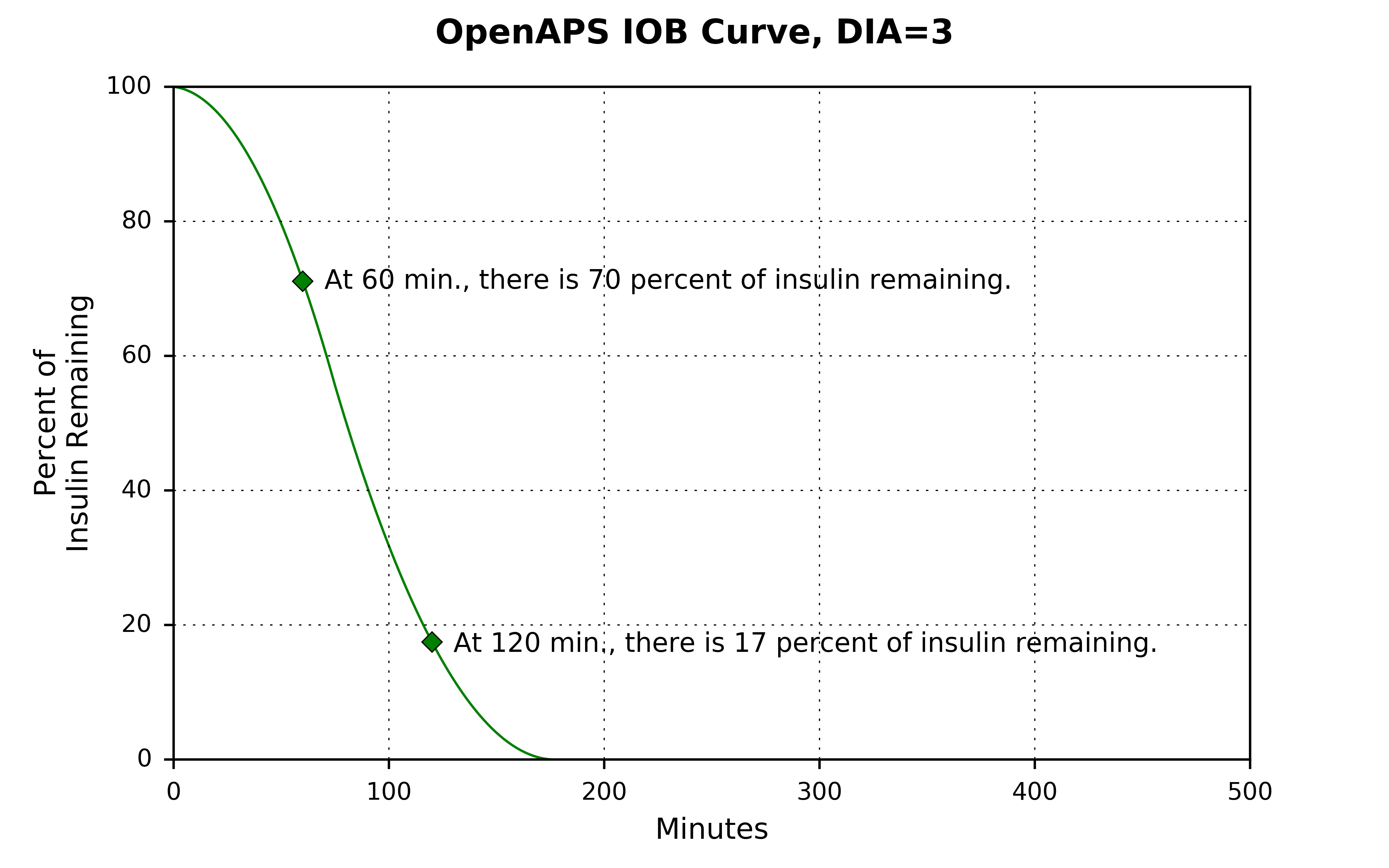
Insulin on Board
Insulin on board (iob), is the inverse of the cumulative activity curves. Instead of ranging from 0 to 100 percent, they range from 100 to 0 percent. With dia set at 3 hours, about 70 percent of insulin is still available an hour after an insulin dosage, and about 17 percent is still available two hours afterwards.
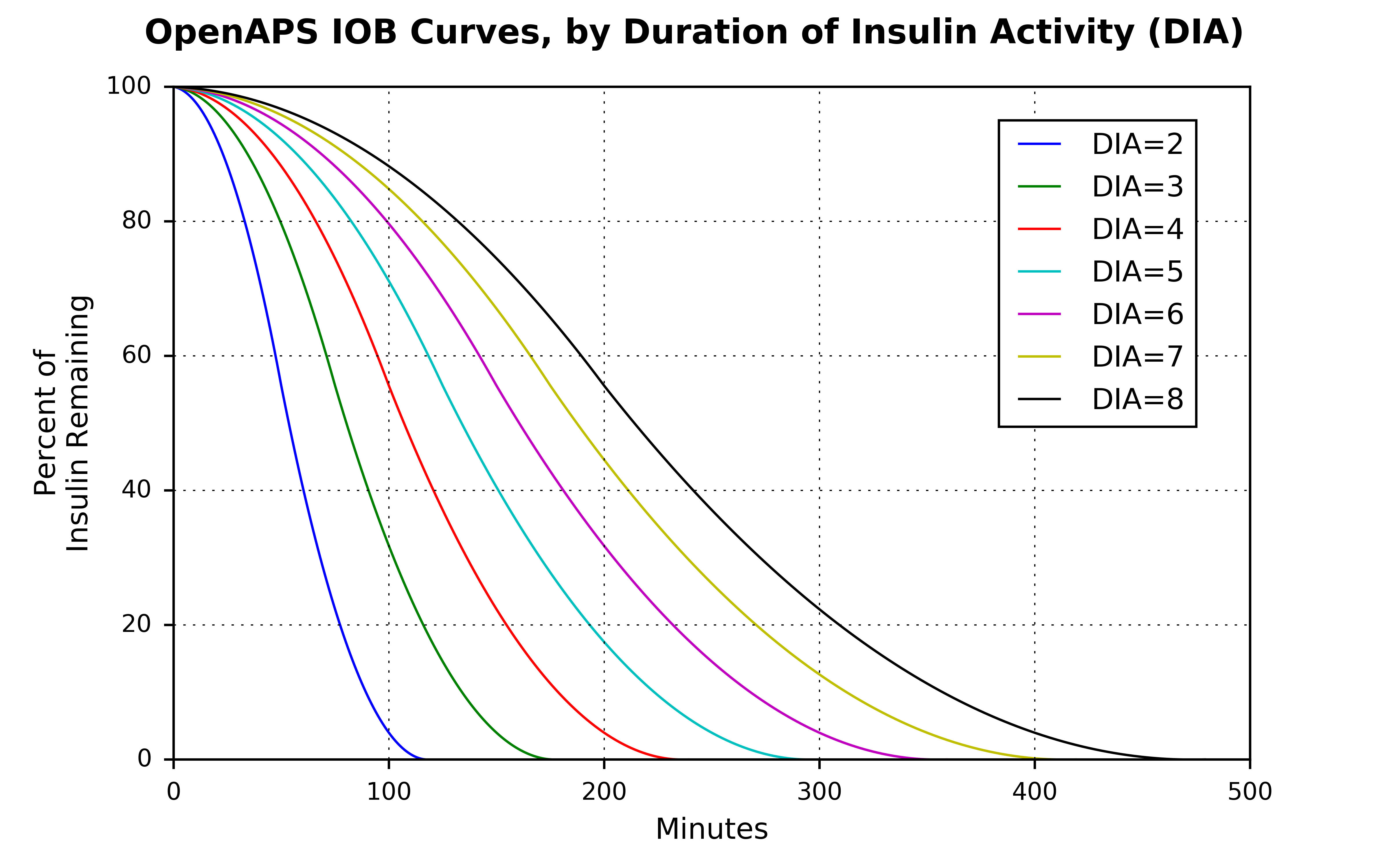
Similar to how the activity “curves” (triangles) and cumulative actvity curves vary by dia settings, the iob curves also vary by dia setting.
Similar to calculations above, the code in oref0/lib/iob/calculate.js calculates a variable called iobContrib, which has two components: treatment.insulin and and a component referenced here as iob. The unit of measurement for treatment.insulin is units of insulin; the unit of measurement for iob is percent of insulin remaining each minute and is used to scale the treatment.insulin value to units of insulin remaining each minute. (There is no variable iob created in oref0/lib/iob/calculate.js. There is, however, a variable called iob created in oref0/lib/iob/total.js, which represents a slightly different concept. See the FINAL NOTE, below, for more details.)
Finally, two sources to benchmark the iob curves against can be found here and here.
A NOTE ABOUT VARIABLE NAMES: A separate program oref0/lib/iob/total.js creates variables named activity and iob. Those two variables, however, are not the same as the activity and iob variables plotted in this documentation page. Those two variables are summations of all insulin treatments still active.
The activity and iob concepts plotted here are expressed in percentage terms and are used to scale the treatment.insulin dosage amounts, so the units for the activityContrib and iobContrib variables are units of insulin per minute and units of insulin remaining at each minute, repectively. Because the activity and iob variables in oref0/lib/iob/total.js are just the sums of all insulin treatments, they’re still in the same units of measurements: units of insulin per minute and units of insulin remaining each minute.
Understanding the New IOB Curves Based on Exponential Activity Curves
As of 0.6.0 OpenAPS has new activity curves available for users to use.
In the new release, users are able to select between using a “bilinear” (looks like what was plotted above: /\) or “exponential” curves. Unlike the bilinear activity curve (which varies only based on dia values in a user’s pump), the new exponential curves will allow users to specify both the dia value to use AND where they believe their peak insulin activity occurs.
A user can select one of three curve defaul settings:
- bilinear: Same as how the curves work in oref0, version 0.5 – IOB curve is calculated based on a bilinear
activitycurve that varies by user’sdiasetting in their pump. - rapid-acting: This is a default setting for Novolog, Novorapid, Humalog, and Apidra insulins. Selecting this setting will result in OpenAPS to use an exponential
activitycurve withpeakactivity set at 75 minutes anddiaset at 300 minutes (5 hours). - ultra-rapid: This is a default setting for the relatively new Fiasp insulin. Selecting this setting will result in OpenAPS to use an exponential
activitycurve withpeakactivity set at 55 minutes anddiaset at 300 minutes (5 hours).
Note: If rapid-acting or ultra-rapid curves are selected, a user can still choose a custom
peakanddiatime, but subject to two constraints:
diamust be greater than 300 minutes (5 hours); if it’s not, OpenAPS will setdiato 300 minutes.peakmust be set between 35 and 120 minutes; if it’s not, OpenAPS will setpeakto either 75 or 55 minutes, depending on whether the user selected rapid-acting or ultra-rapid default curves.
What Do The Exponential Curves Look Like?
Most commonly, exponential is associated with exponential growth – as in, how quickly bacteria might grow in a petri dish, for example. A little less commonly, exponential is associated with exponential decay – as in, what the radioactive half-life of a particular element might be.
Examples of such exponential growth and exponential decay could look like this:
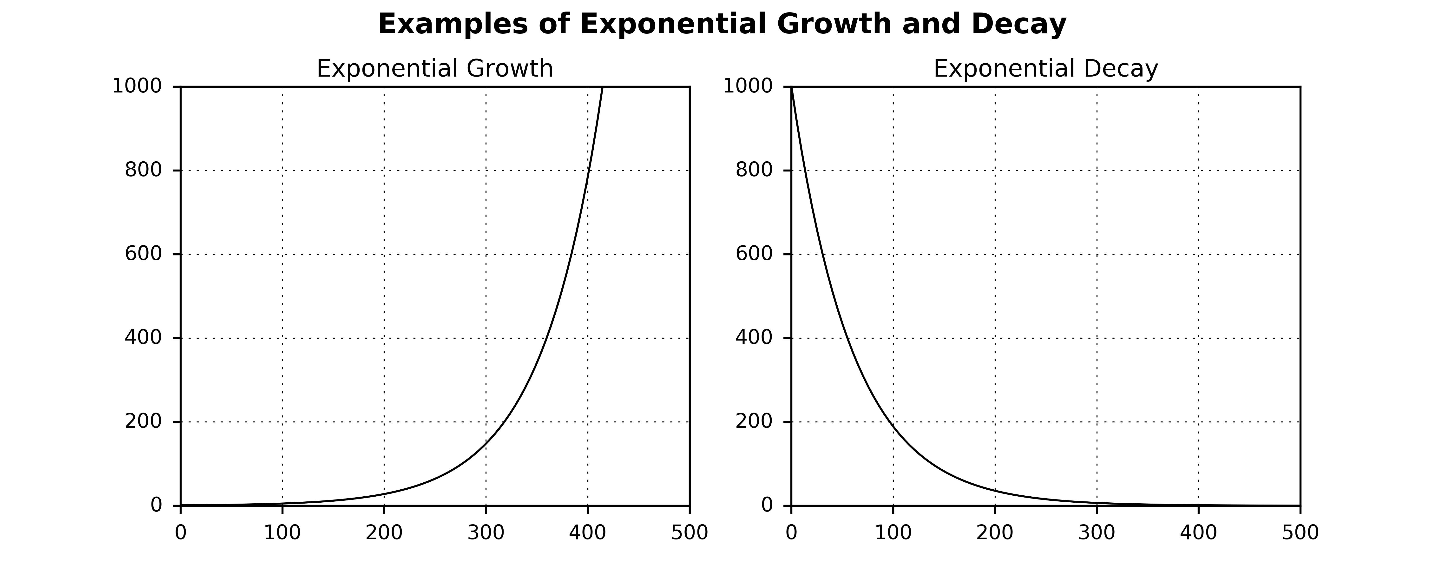 (Though the mathematical formulas can be written such that how steep the growth or decay curves can vary quite a bit.)
In the application of exponential curves in modeling how insulin is used in the human body, the trick is to write a mathematical formula that combines some delay in the activity, some rapid growth in the activity to the peak, and then a smooth transition down until all the insulin is used up. (See the Technical Details, below for links to the underlying math.)
With dia set to 5 hours and the peak set to 75 minutes (the default settings for rapid-acting insulins), the exponential activity curves in the OpenAPS dev branch looks like this:
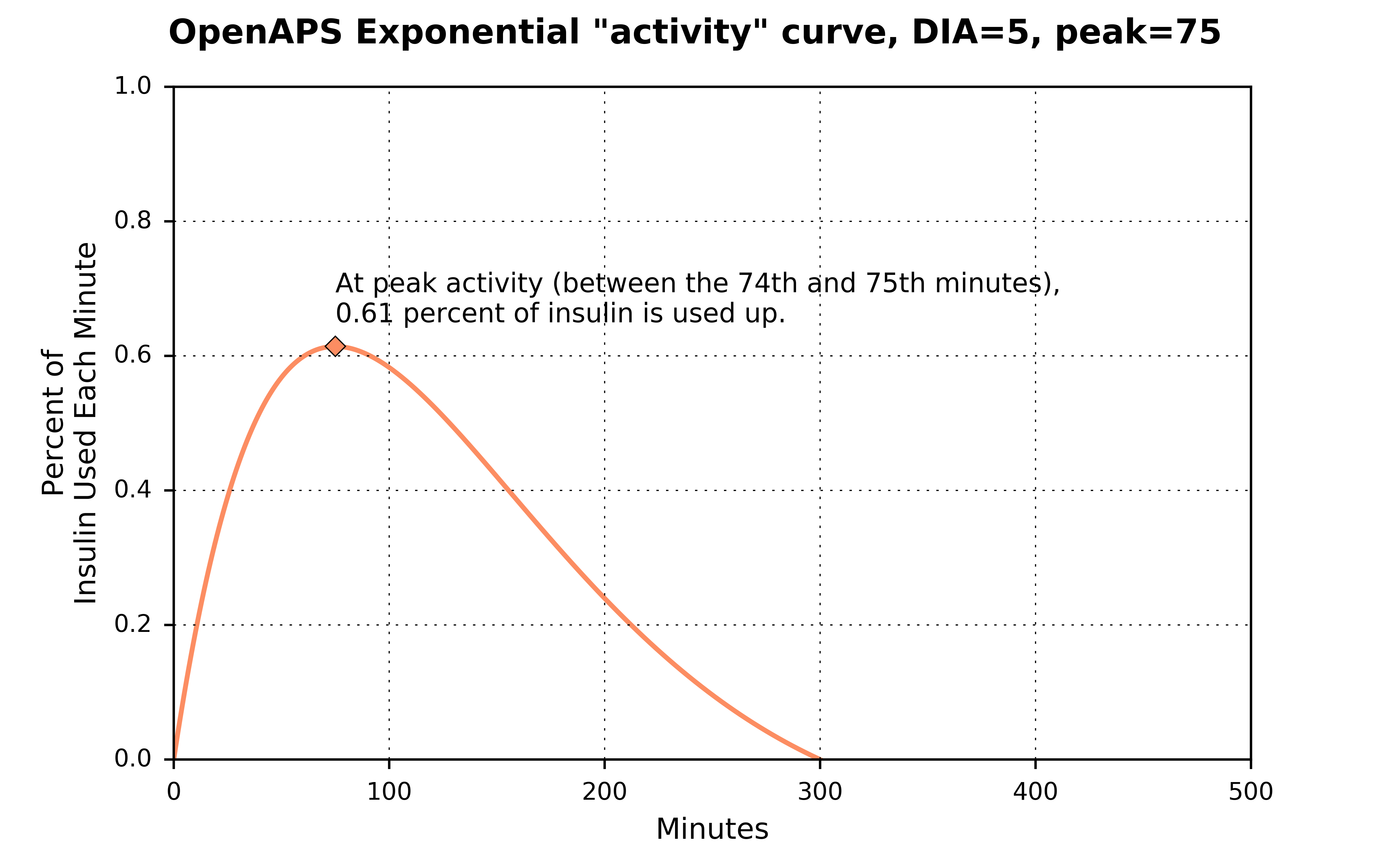
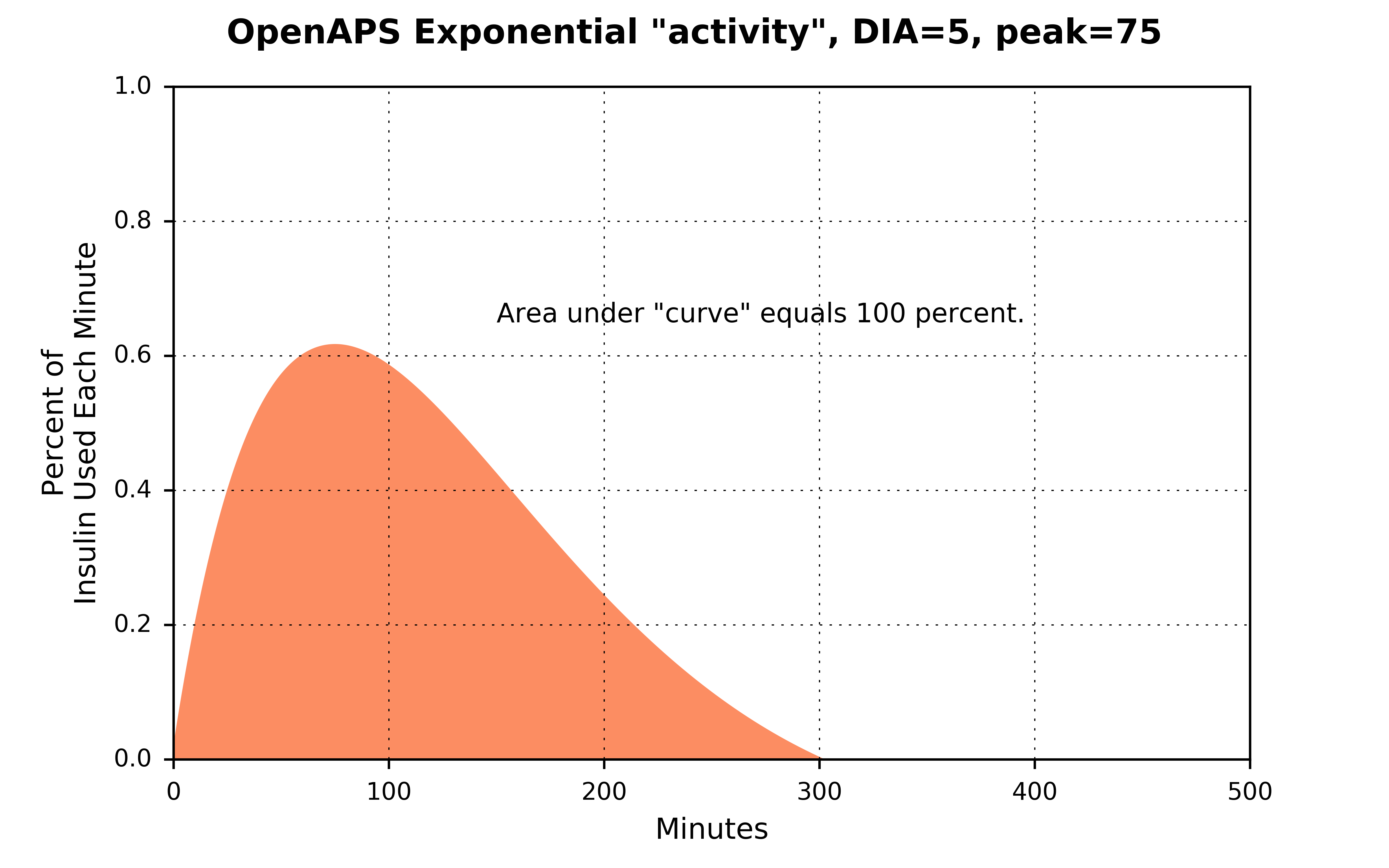
Just like how the bilinear curve in OpenAPS version 0.5.4, the activity curves in version 0.6 will start at zero and end at zero and the area under the curve will sum up to 100 percent of the insulin being used up.
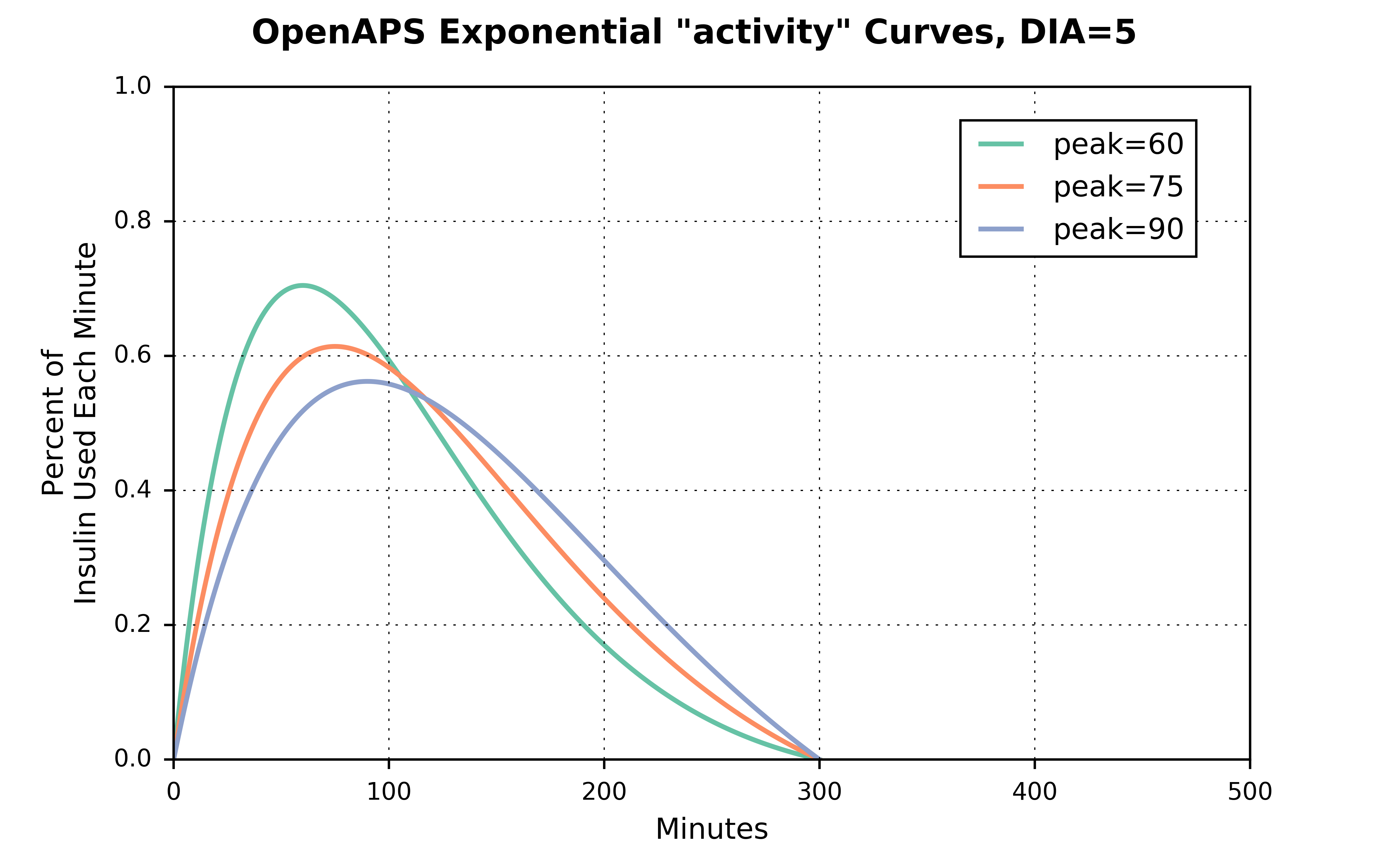
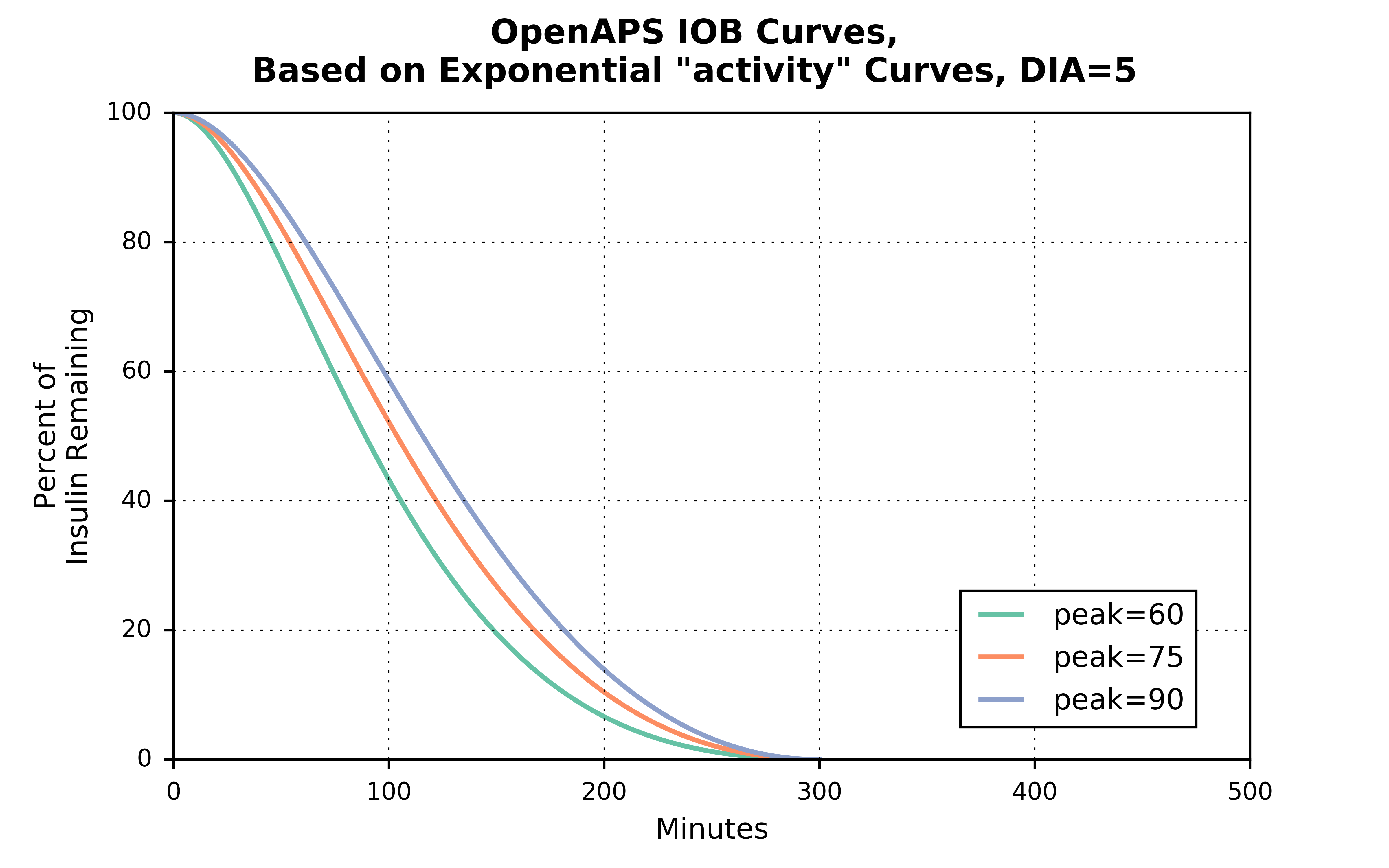
The shape of exponential activity curves can vary by either dia or by peak. Below is what the activity curves look like for three separate peak settings, but holding the dia setting fixed at 5 hours.
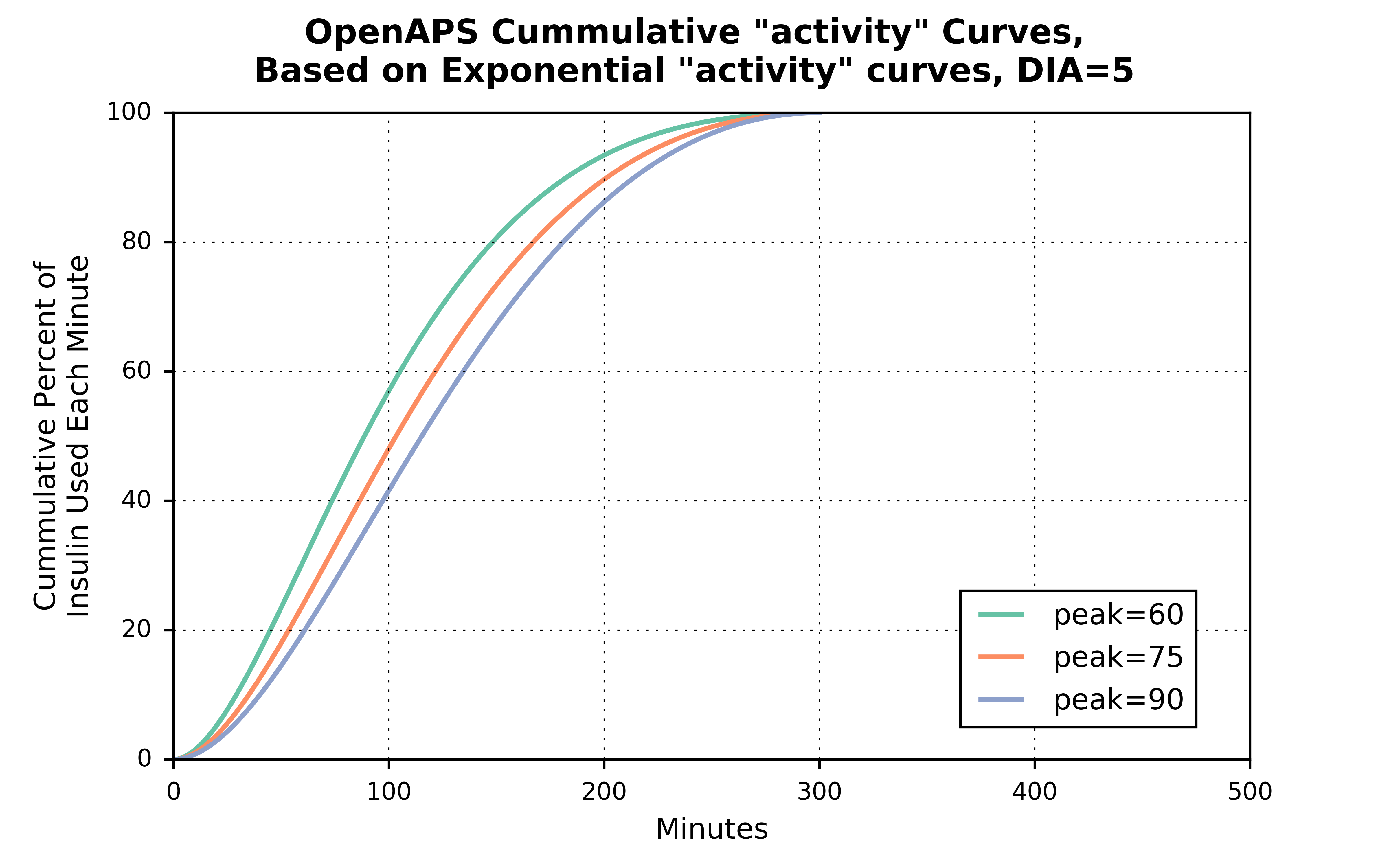
A useful way to visualize how the activity curves translate to the iob curves is to first show what the cumulative activity curves look like:
And then the iob curves are just the inverse of the cumulative activity curves:
How Do The Exponential Curves Compare To The Bilinear Curves?
The most important question to a user might be: “Well which set of curves is better for me to use?”
Everyone is different, and their bodies may absorb insulin at different rates. Furthermore, an individual’s insulin absorption may vary from day-to-day or week-to-week for many reasons. But with a lot of parameter settings, finding the best one is often a process of trial-and-error.
That said, the bilinear curve currently used in OpenAPS 0.5.4 is a relatively simple model of how insulin is absorbed. Although it’s a simple model, in many cases it provides decent approximations. The proposed exponential curves are more complex and more closely aligned to how an individual’s body might absorb their insulin. But users may or may not find significant differences in how their OpenAPS performs just by switching to the exponential curves.
You can think of the exponential curve for the default rapid-acting insulin settings (dia = 5 hours, peak = 75 minutes) as being a combination of two bilinear curves. One where dia is set to 3 hours and the peak occurs at 75 minutes; and another one where the dia is set to 5 hours, but the peak occurs at 125 minutes.
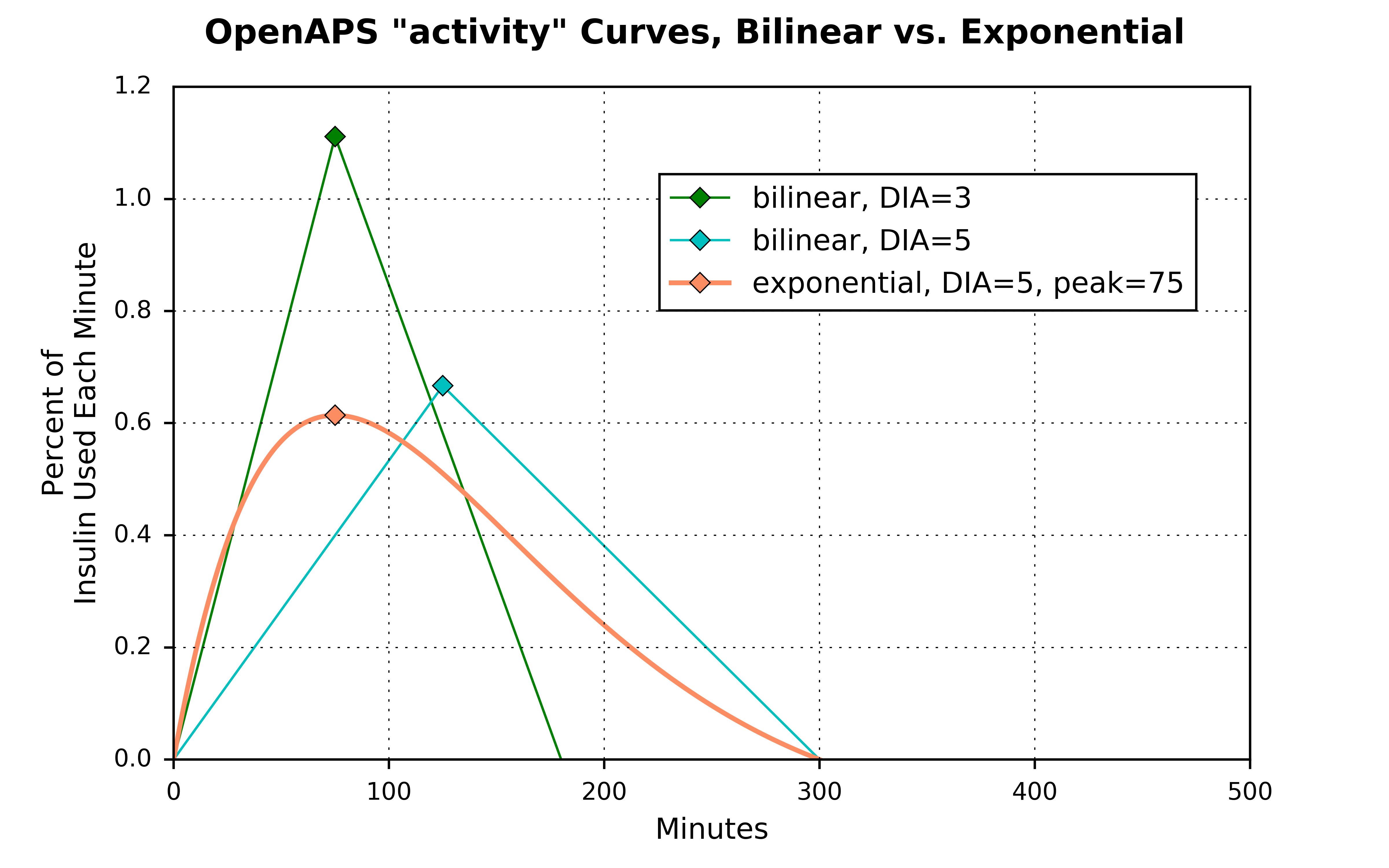 (The area under each of the three curves sums to 100 percent.)
To make a more direct, apples-to-apples, comparison, setting the exponential curve with dia = 5 hours and peak = 125 minutes, the difference between the two curves is a little clearer:
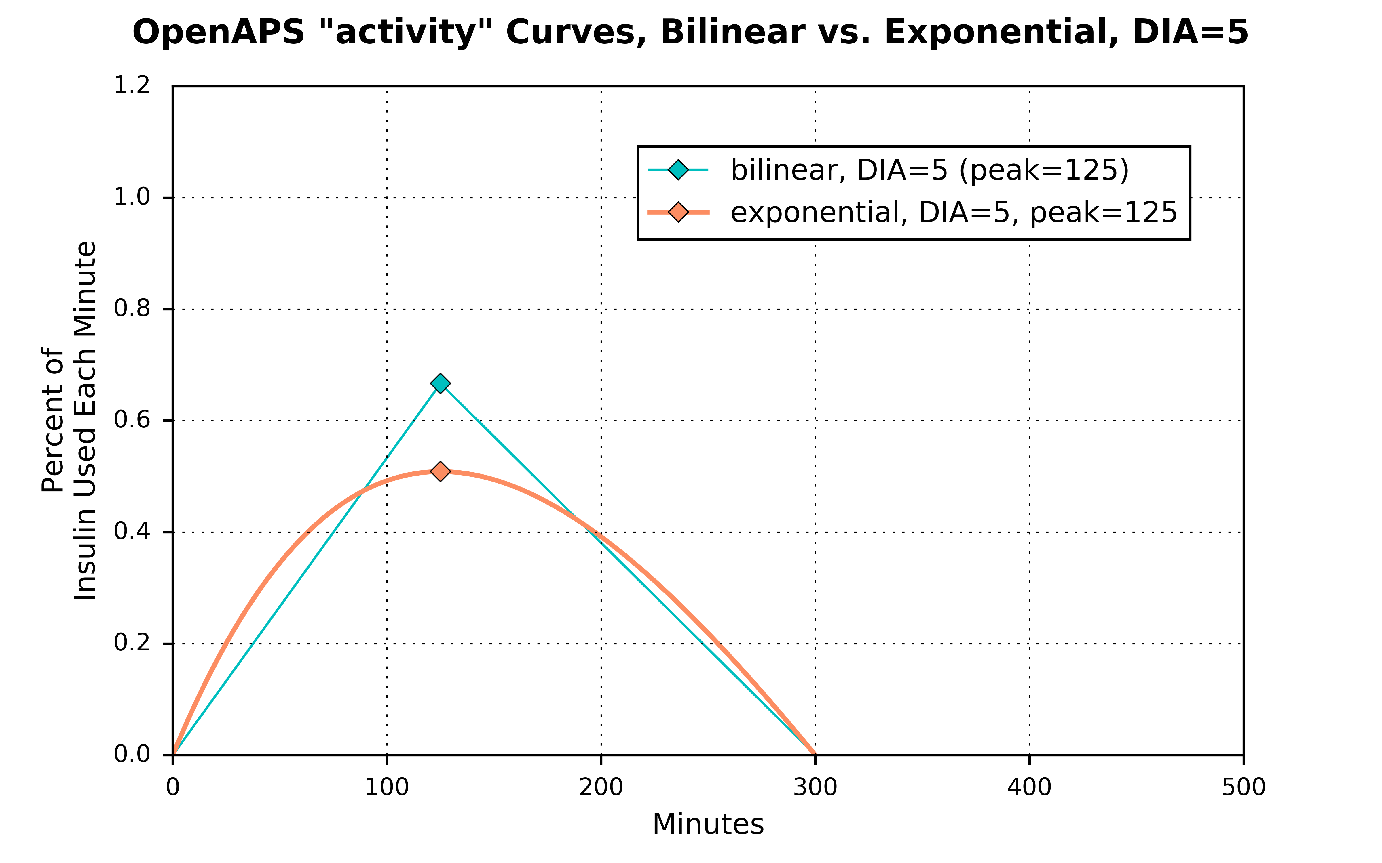 NOTE: As described above, OpenAPS will NOT allow you to set a
 peak value above 120 minutes. This graph is shown just to make a direct comparison between the two types of curves.
Finally, going back to an exponential curve with dia set to 5 hours and peak set to 75 minutes, the comparison between how the iob curve looks relative to the iob curve using the bilinear activity curve with dia set to 5 hours is probably the most relevant:
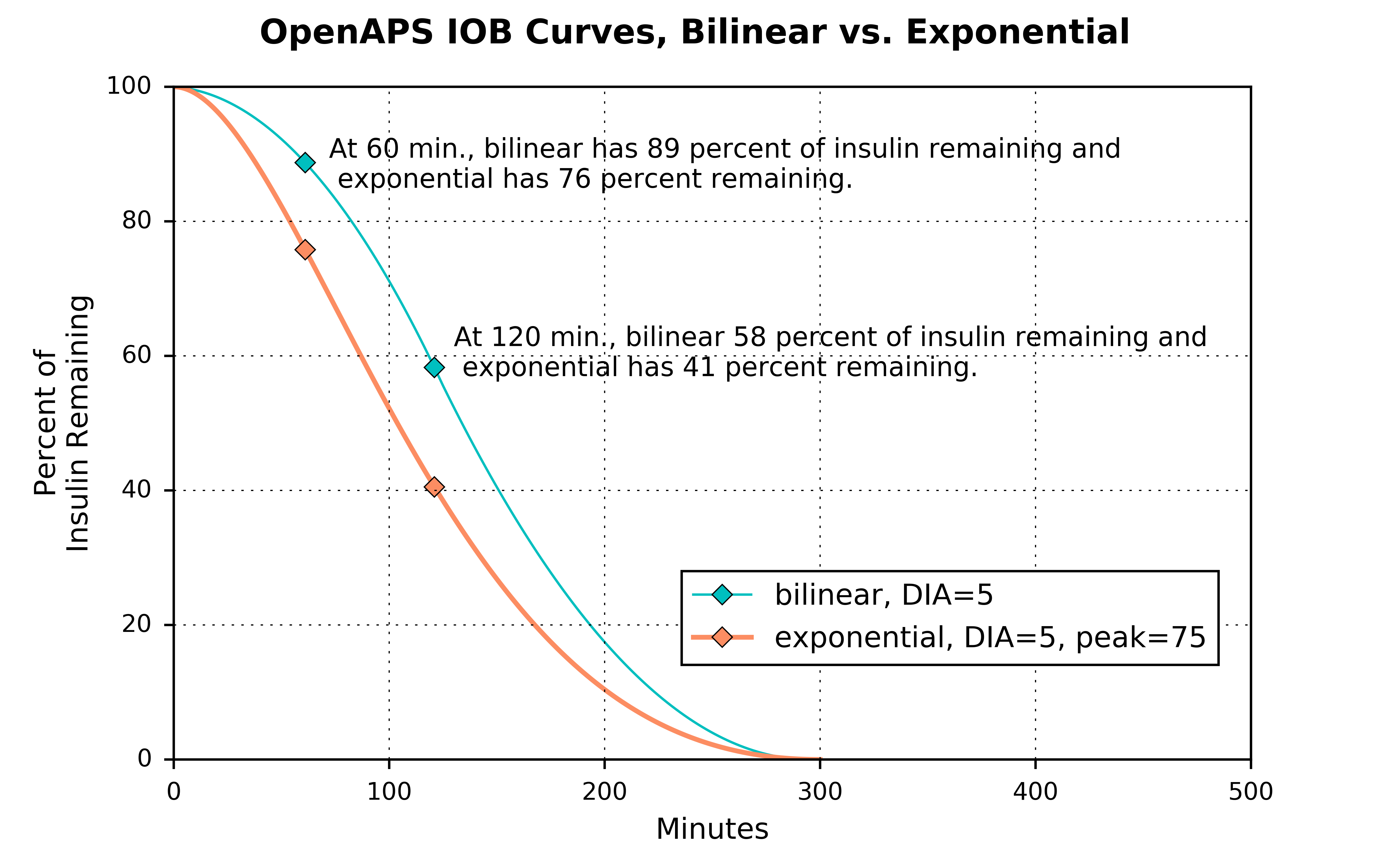
The iob curve based on the exponential activity curve has insulin being used up significantly faster than the iob curve based on the bilinear activity curve. After one hour, for example, there is a 13 percent difference in how much insulin is remaining between the two curves, and after 2 hours there is a 17 percent difference between the two curves.
Technical Details
The source for the new functional forms for the exponential curves were calculated by Dragan Macsimovic and can be found as part of a discussion on the LoopKit Github page. There were many others contributing to this discussion, development, and testing of exponential curves for Loop and OpenAPS. The full discussion is very technical, but useful if you want more information on the exponential curves.